How Good is the Approximation?
In the above example, notice how \(f(1)=1\) and that the approximation \(L(1)=-1+2\implies L(1)=1\). The approximation is exactly on with the function value, but this does not always happen. The following table outlines some details involving underestimates and overestimates:
| Underestimates | Overestimates |
|---|---|
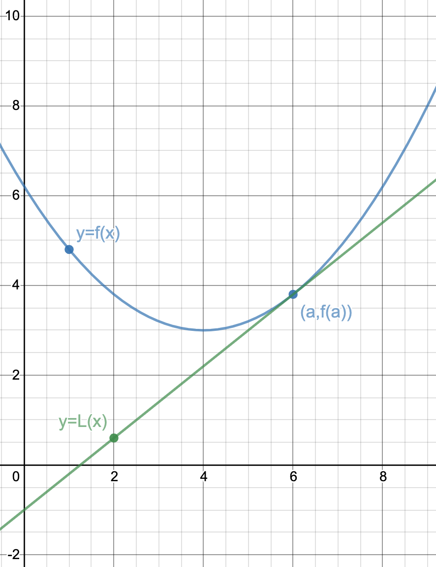
| The graph shows \(f(x)\) above \(L(x)\) near \(x=a\). | The graph shows \(f(x)\) below \(L(x)\) near \(x=a\). |
 |
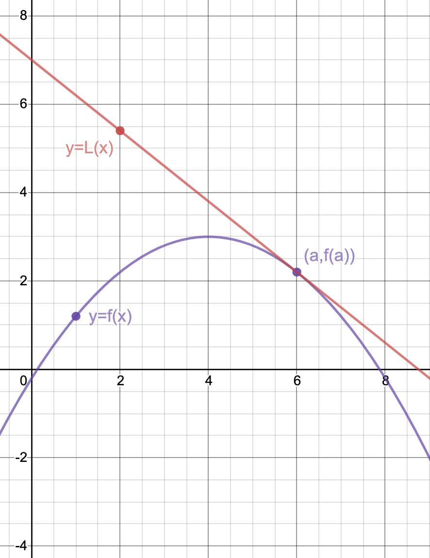 |
| The function is concave up near \(x=a\), making \(L\) an underestimate to \(f\). | The function is concave down near \(x=a\), making \(L\) an overestimate to \(f\). |
The concavity of the function will also determine how good the approximation can be. If the graph has concavity with more curvature, then the function will move away from \(L(x)\) more quickly causing more error in the approximation. If the graph has concavity with less curvature, then the function will remain close to \(L(x)\) causing smaller error in the approximation.
Example
Find the linear approximation to \(f(x)=e^{-x}\) at \(x=\ln2\). Use the approximation to estimate \(e^{-0.7}\). Is it an overestimate or an underestimate?
| Find the linear approximation: | \(\displaystyle{\begin{array}{l} f(\ln2)=e^{-\ln2} \\ \implies f(\ln2)=e^{\ln2^{-1}} \\ \implies f(\ln2)=2^{-1} \\ \implies f(\ln2)=\frac{1}{2}\end{array}}\) | \(\displaystyle{\begin{array}{l} f^\prime(x)=-e^{-x} \\ \implies f^\prime(\ln2)=-e^{-\ln2} \\ \implies f^\prime(\ln2)=-e^{\ln2^{-1}} \\ \implies f^\prime(\ln2)=2^{-1} \\ \implies f^\prime(\ln2)=\frac{1}{2}\end{array}}\) |
| The linear approximation becomes: \(\displaystyle{L(x)=\frac{1}{2}-\frac{1}{2}(x-\ln2)}\). | ||
| Estimate \(e^{-0.7}\) using \(L(x)\): | \(\displaystyle{\begin{array}{l} L(0.7)=\frac{1}{2}-\frac{1}{2}(0.7-\ln2) \\ \implies L(0.7)\approx0.4965735903\end{array}}\) | The value of \(f(0.7)\) from a calculator is: \(0.4965853037\), which agrees with the approximation to \(4\) decimal places. |
| From the calculation, it's clear that the approximation is an underestimate. How can that be determined without looking at the value of \(f(0.7)\)? Use concavity of \(f\) by looking at the second derivative. | ||
| Second derivative: \(f^{\prime\prime}(x)=e^{-x}\). | For all values of \(x\), especially near \(x=\ln2\), \(f^{\prime\prime}(x)>0\). This means \(f(x)\) will be concave up near \(x=\ln2\) meaning the approximation will be an underestimate. | |