Algebra 1 - Systems of Linear Equations: Graphing Method
It makes sense that when looking at a system of linear equations, that if one graph could show both lines, then a lot can be determined about the solution to the system. Look at the following graphs to see the types of solutions possible by different systems:
Exactly One Solution
No Solutions
Infintely Many Solutions
As the graphs show, a system can have three possible outcomes: #1 exactly one solution, #2 no solutions and #3 an infinite number of solutions. This is a really nice feature of using the graphing method, it provides a visual representation of the solutions. To be successful with the graphing method, each linear equation must be graphed correctly. The following examples will show how to implement the graphing method to solve a system of linear equations.
Example (Slope-intercept Form)
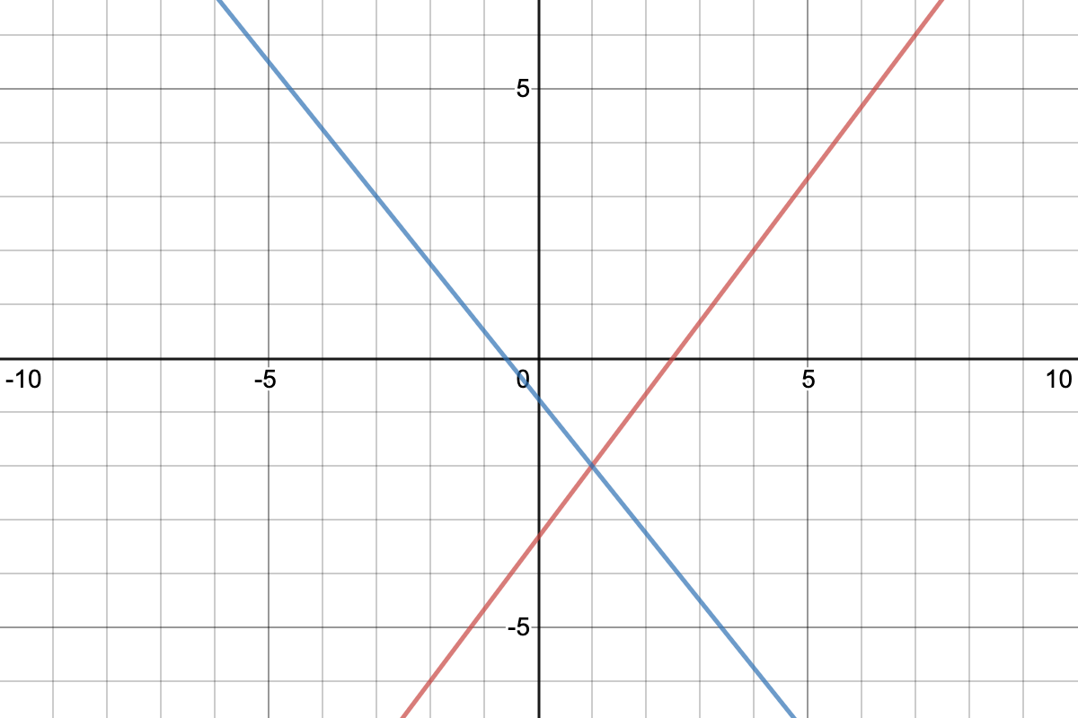
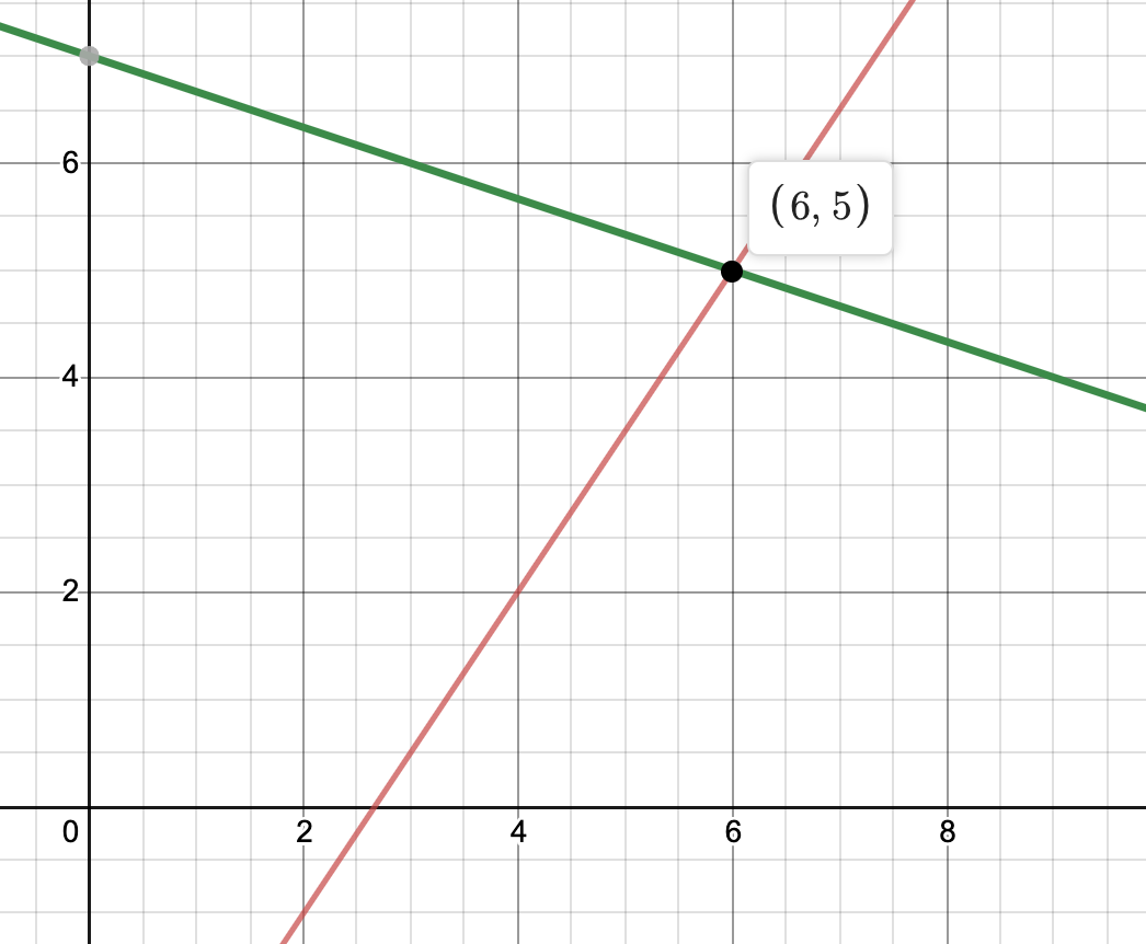
Use the graphing method to find the solution to the system: \(\begin{array}{c} y=\large{\frac{3}{2}}\normalsize{x-4} \\ y=\,-\large{\frac{1}{3}}\normalsize{x+7} \end{array}\).
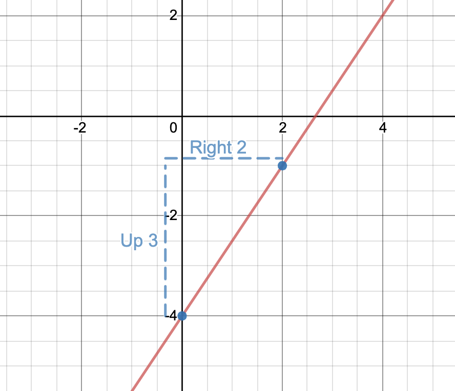
Solution To graph \(y=\large{\frac{3}{2}}\normalsize{x-4}\), recall the \(y\)-intercept is at the point \((0,-4)\). Using the slope of \(\large{\frac{3}{2}}\), from \((0,-4)\) move up 3 and to the right 2, making a second point at \((2,-1)\). Now draw the line extending through these two points:
Using the same technique to graph the second line, the graph looks like:
From reading the graph, the solution is at the point: \((6,5)\).
The next example has one equation in point-slope form. Use the same graphing methods as slope-intercept, except at a different starting point.
Example (Point-slope Form)
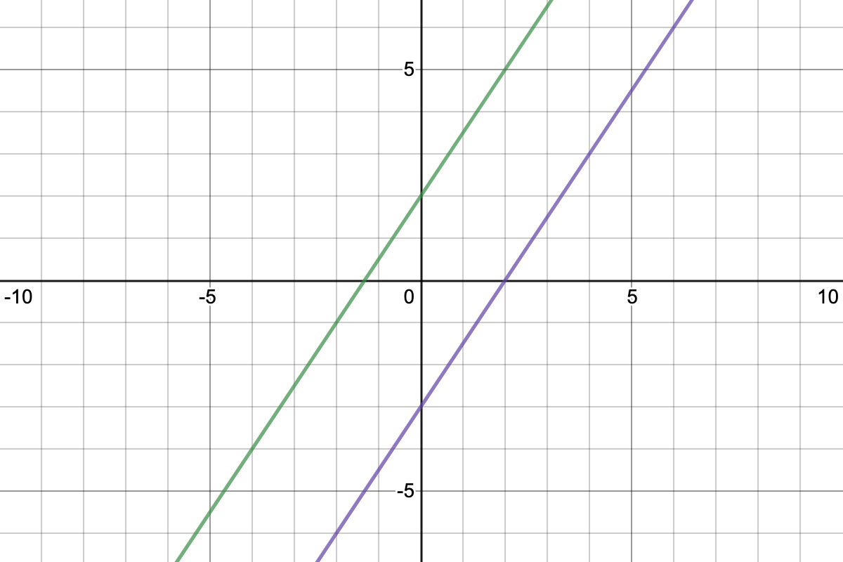
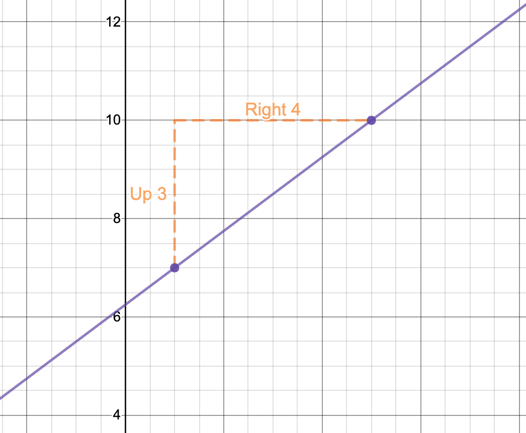
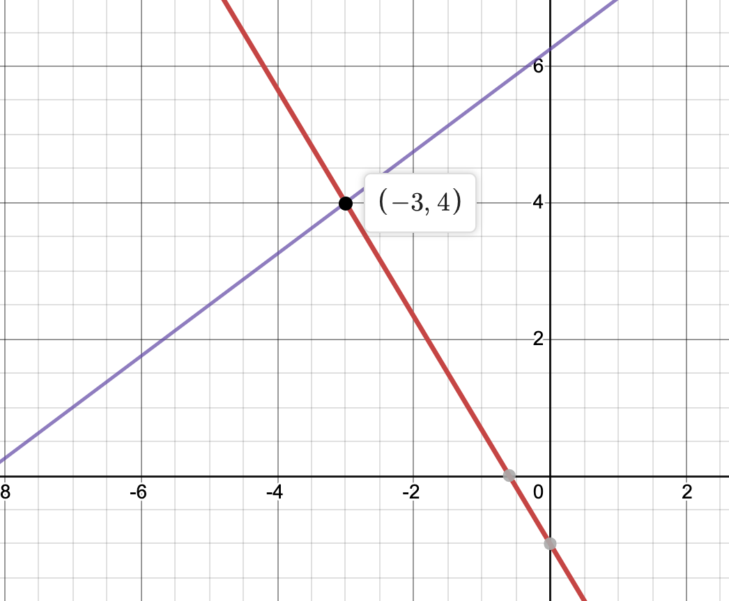
Use the graphing method to find the solution to the system: \(\begin{array}{c} y=\,-\large{\frac{5}{3}}\normalsize{x-1} \\ y-7=\large{\frac{3}{4}}\normalsize(x-1) \end{array}\).
Solution The first equation is in slope-intercept form, see the previous example on how to graph. To graph \(y-7=\large{\frac{3}{4}}\normalsize{(x-1)}\), recall the point-slope equation has the point given in it, here the point is \((1,7)\). Now start at this point and use the slope of \(\large{\frac{3}{4}}\) like before, the second point is at \((5,10)\). Now draw the line extending through these two points:
Once the graph of the second line is added, the graph looks like:
From reading the graph, the solution is at the point: \((-3,4)\).
The last example is when a system involves an equation in standard form. The procedure for graphing from this form is to find the intercepts.
Example (Standard Form)
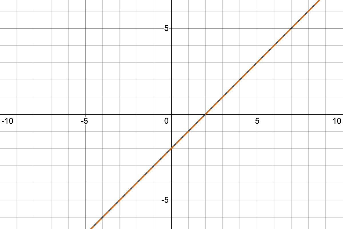
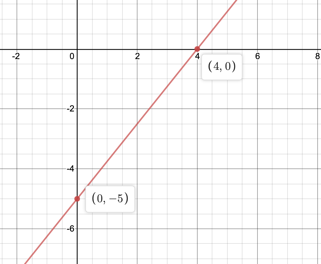
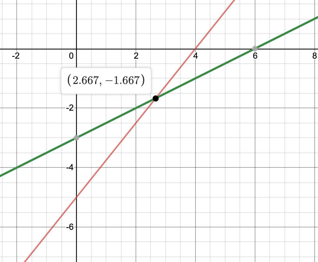
Use the graphing method to find the solution to the system: \(\begin{array}{c} 5x-4y=20 \\ -6x+12y=-36 \end{array}\).
Solution To find the intercepts, replace one variable with 0 and solve for the other.
Now draw the line extending through these two points:
Once the graph of the second line is added, the graph looks like:
From reading the graph, the solution is at the point: \((2.667,-1.667)\).
CAUTION: The last example shows something that occurs sometimes with systems of linear equations. The solution involves decimals, or fractions. When using the graphing method, it may be difficult to read off the solution when decimals or fractions occur. The use of technology, such as Desmos, is vital for helping find solutions like these.